

4.2 MTF & Sharpness
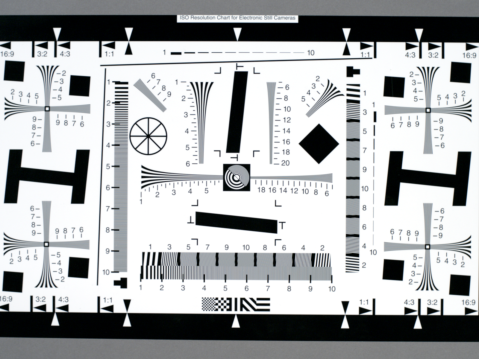
ISO 12233
Modulation Transfer Function
The ISO 12233 Chart is a very useful tool to help measure camera system MTF and Sharpness. Every element in a camera system will affect the sharpness and resolving power of the image. Testing this between two different camera systems can add a lot of variability. Not only are you testing the camera sensor with film, but in addition the camera lens as well. In best practices, each camera should be tested with the same lens, and with several lenses. This will make it easier to separate the lens MTF from the camera MTF.
MTF:
Without going into too much detail about what MTF is, if you look at the chart and take note of the high frequency black and white portions of the chart; at some point, because of how close the lines are together it will appear gray. The less MTF degradation, the less gray will appear, which means the black lines can be seen.
Some of the lines that curve out on the end, appear to be a full line, but as you move further down the lines, the harder it is to follow because they sort of start to mesh together.
To learn more about MTF
The normal exposures for each camera are shown below:


The MTF curves shown in this section were generated from the slant edges in the ISO 12233 chart. Images of this chart were captured for each camera at a
Normal Exposure
+2 Stops Overexposed
-2 Stops Underexposed
Both vertical and horizontal MTFs were calculated for each condition as well. The images were first linearized using the inverse of the calculated OETF curves, then scaled to 8-bit space. The MTF curves were then generated using the sfrmat3 Matlab program by Peter Burns.
The resulting MTF curves for these are:


Comparing the D21 curves vs. the Film curves show that film performs significantly better than the D21 at low frequencies, but only slightly better at higher frequencies.
The film’s sharpness drops very quickly at around 0.05 cycles/pixel, down to only about 10% of the performance at 0.15 cycles/pixel.
The D21, in contrast, loses sharpness much more gradually. It doesn’t hit the 10% mark until around 0.5 cycles/pixel, the half-sampling mark.
The aesthetic result of this is that the images from the D21 appear sharper than those from the film. Since the D21 preserves more contrast at higher frequencies, edges will appear crisp and clean, while those captured on film will appear softer and slightly blurred. This can be observed in the test scene below.
MTFs Were Generated For The Underexposed Images. The Original Images Captured Are Shown Below:


Noise is a major source of error in these measurements. It is difficult to determine the exact performance of the film at any frequency below about 0.2 cycles per degree because the data is so noisy.
The blue channel in particular is the most noisy. The general shape of the curve can be determined, but it is impossible to choose a number to represent this. There is also potential for lens blurring on this particular shot which causes the shot to looks out of focus. The difference in lenses used may be cause for additional error.


The Generated MTF Plots From These Images Are:


The D21 footage is significantly noisier for the underexposures than the normal exposures, which disrupts the data.
However, it clear that the D21 continues to perform much better than the film at mid-to-high frequencies.
Comparing the D21 plots to those from the normal exposure, the underexposed images represent a slight decrease in performance from the normal exposures.
Now, the modulation reaches the 10% point a bit sooner, at around 0.4 cycles/pixel, compared to the 0.5 from before. This is to be expected. The overall modulation of the image has decreased since the whites are dimmer but the blacks remain at close to the same level.
The result is that when an image is underexposed, it may appear slightly softer than one at a normal exposure. The film appears to perform about the same as it did previously. Again, the data is quite noisy, so it is difficult to determine exact numbers, but the MTF hits approximately 10% at around 0.15 to 0.2 cycles/pixel. This is likely due to the dynamic range of the film. This helps preserve the overall modulation and contrast. So, the film performs similarly whether it was properly exposed or not. Finally, the overexposed test images are given below:
MTFs Were Generated For The Overexposed Images. The Original Images Captured Are Shown Below:


The Calculated MTF Plots Are Shown Below:


For the overexposures, the D21 again performs slightly worse than for the normal exposures, but better than it did for the underexposures.
The slope of the plots are a bit steeper, and they hit the 10% point at an average of 0.45 cycles/pixels.
This failure is caused by the same factor as the underexposed images. The entire image is brighter, including the black portions, which decreases the overall modulation.
The reason it performs better overexposed than underexposed is because overexposure uses smaller grains and so are generally better because of effective resolution gains!
The film appears to have performed better when overexposed than in either of the other two cases. The vertical MTF plot shows this increase by a significant amount, hitting 10% modulation at around 0.3 cycles/pixel. However, the horizontal plot looks more similar to those of the previous two exposures. The difference between these is likely a result of noise differences in the two regions of the image where the slant edges lie.
The horizontal MTF appears to be more accurate based off its similarity to the other film plots. In this case, the film is a bit sharper when overexposed, and this is likely due to the dynamic range of the film as well as the linearization.
The film is already better at preserving modulation when not properly exposed, and the increase after linearizing the data only gives it more of an advantage.
Aliasing
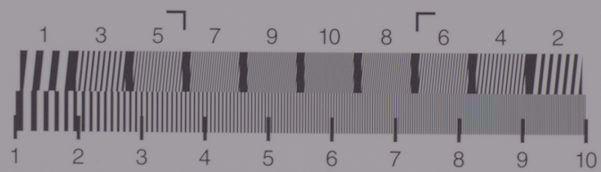
Fig 16.1 D21 Aliasing Example
Aliasing occurs when a high frequency pattern is sampled below the Nyquist rate, that is, at two samples per cycle, producing a low frequency artifact. This happens often in digital imaging systems whose fixed pixel size can only reproduce patterns up to a certain frequency. This effect is evident in the footage shot by the D21.
As the frequency of the pattern increases on this area of the ISO 12233 chart a wave pattern can be seen. It starts to become the most noticeable in patch 6 of both the top and bottom row.
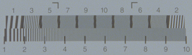
Fig 16.2 Film Aliasing Example
As an analog system, film does not suffer from aliasing. Instead of producing a wave pattern as was seen with the D21, areas of high frequency just blend together. This is because unlike digital systems, film grains are of varying sizes, and are scattered in a random arrangement throughout the film. Aliasing patterns can only occur when the light-detecting elements are arranged in a perfect grid to form uniform, low-frequency patterns.
However, even though the film itself will not produce aliasing the scanner used to transfer film uses a digital sensor. As a result, aliasing can still be found in footage that was originally shot on film. In our footage, there is no apparent aliasing in the film. Because we scanned the film at 4K resolution, the pixels are smaller than many of the film grains, so the image is visibly the same as it would have been viewing the film in an analog format. Furthermore, the film footage was very noisy, and not as sharp as the D21, both of which help to cover up any aliasing artifacts that could have occurred.
“Because we scanned the film at 4K resolution, the pixels are smaller than many of the film grains, so the image is visibly the same as it would have been viewing the film in an analog format.”